Eigenvalue distribution of Gaussian orthogonal random matrices¶

The eigenvalues of random matrices obey certain statistical laws. Here we construct random matrices from the Gaussian Orthogonal Ensemble (GOE), find their eigenvalues and then investigate the nearest neighbor eigenvalue distribution \(\rho(s)\).

[1]:

from rmtkernel import ensemble_diffs, normalize_diffs, GOE
import numpy as np
import ipyparallel as ipp

Wigner’s nearest neighbor eigenvalue distribution¶

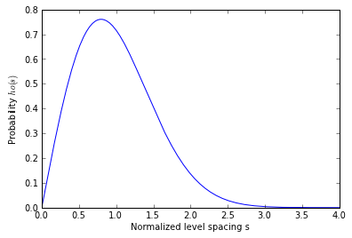
The Wigner distribution gives the theoretical result for the nearest neighbor eigenvalue distribution for the GOE:

\[\rho(s) = \frac{\pi s}{2} \exp(-\pi s^2/4)\]

[2]:

def wigner_dist(s):
    """Returns (s, rho(s)) for the Wigner GOE distribution."""
    return (np.pi*s/2.0) * np.exp(-np.pi*s**2/4.)

[3]:

def generate_wigner_data():
    s = np.linspace(0.0,4.0,400)
    rhos = wigner_dist(s)
    return s, rhos

[4]:

s, rhos = generate_wigner_data()

[17]:

plot(s, rhos)
xlabel('Normalized level spacing s')
ylabel('Probability $\rho(s)$')

[17]:

&lt;matplotlib.text.Text at 0x3828790&gt;

Serial calculation of nearest neighbor eigenvalue distribution¶

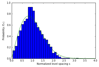
In this section we numerically construct and diagonalize a large number of GOE random matrices and compute the nerest neighbor eigenvalue distribution. This comptation is done on a single core.

[6]:

def serial_diffs(num, N):
    """Compute the nearest neighbor distribution for num NxX matrices."""
    diffs = ensemble_diffs(num, N)
    normalized_diffs = normalize_diffs(diffs)
    return normalized_diffs

[7]:

serial_nmats = 1000
serial_matsize = 50

[8]:

%timeit -r1 -n1 serial_diffs(serial_nmats, serial_matsize)

1 loops, best of 1: 1.19 s per loop

[9]:

serial_diffs = serial_diffs(serial_nmats, serial_matsize)

The numerical computation agrees with the predictions of Wigner, but it would be nice to get more statistics. For that we will do a parallel computation.

[10]:

hist_data = hist(serial_diffs, bins=30, normed=True)
plot(s, rhos)
xlabel('Normalized level spacing s')
ylabel('Probability $P(s)$')

[10]:

&lt;matplotlib.text.Text at 0x3475bd0&gt;

Parallel calculation of nearest neighbor eigenvalue distribution¶

Here we perform a parallel computation, where each process constructs and diagonalizes a subset of the overall set of random matrices.

[11]:

def parallel_diffs(rc, num, N):
    nengines = len(rc.targets)
    num_per_engine = num/nengines
    print "Running with", num_per_engine, "per engine."
    ar = rc.apply_async(ensemble_diffs, num_per_engine, N)
    diffs = np.array(ar.get()).flatten()
    normalized_diffs = normalize_diffs(diffs)
    return normalized_diffs

[12]:

client = ipp.Client()
view = client[:]
view.run('rmtkernel.py')
view.block = False

[13]:

parallel_nmats = 40*serial_nmats
parallel_matsize = 50

[14]:

%timeit -r1 -n1 parallel_diffs(view, parallel_nmats, parallel_matsize)

Running with 10000 per engine.
1 loops, best of 1: 14 s per loop

Parallel Monto-Carlo options pricing Futures in IPython Parallel